Midterm Checkpoint
Introduction
Accurate house pricing is essential in the real estate and mortgage industries, influenced by physical attributes and neighborhood characteristics. Research has explored various machine learning techniques for house price prediction. A study titled “An Optimal House Price Prediction Algorithm: XGBoost” compared algorithms such as XGBoost, Support Vector Regressor, Random Forest Regressor, Multilayer Perceptron, and Multiple Linear Regression using the Ames City housing dataset. XGBoost was identified as the most effective model, offering interpretability, simplicity, and accuracy [3].
The dataset we used was a set of listings scraped from realtor.com, focusing on houses sold within the past 10 years in the following zip codes in Georgia: 30097, 30096, 30022, 30005. This dataset includes features like sell price, property location, year built, bedrooms, bathrooms, and other amenities crucial for pricing. Location details will assist in future regional analysis [1].
Problem Definition
In Georgia’s fluctuating real estate market, accurately pricing a house is a complex challenge. Traditional valuation methods, such as comparative market analysis, often overlook essential details and lack critical context [2]. This results in homes being frequently mispriced, leading to discrepancies in their market value. Moreover, obtaining more accurate valuations can be both time-consuming and costly. This project seeks to address these limitations by leveraging machine learning models, which can analyze vast amounts of data to provide more precise and reliable property valuations.
Methods
First, we cleaned the data by removing duplicate listings and replacing null values. During the preprocessing step, we selected features that could be numerically represented for the training step. Out of the 29 columns of the original dataset, we reduced 12 relevant features. Features such as state and status were removed because their variances were 0. Irrelevant features such as mls_id, property_url, and primary_photo were also removed. Location features such as city and street were removed because longitude and latitude were already provided.
The following table represents the remaining features after cleaning:
| # | Column | Non-Null Count | Dtype |
| 0 | style | 21338 non-null | object |
| 1 | beds | 21338 non-null | float64 |
| 2 | full_baths | 21338 non-null | float64 |
| 3 | half_baths | 21338 non-null | float64 |
| 4 | sqft | 21338 non-null | float64 |
| 5 | year_built | 21338 non-null | float64 |
| 6 | list_date | 21338 non-null | object |
| 7 | sold_price | 21338 non-null | int64 |
| 8 | lot_sqft | 21338 non-null | float64 |
| 9 | latitude | 21338 non-null | float64 |
| 10 | longitude | 21338 non-null | float64 |
| 11 | stories | 21338 non-null | float64 |
| 12 | parking_garage | 21338 non-null | float64 |
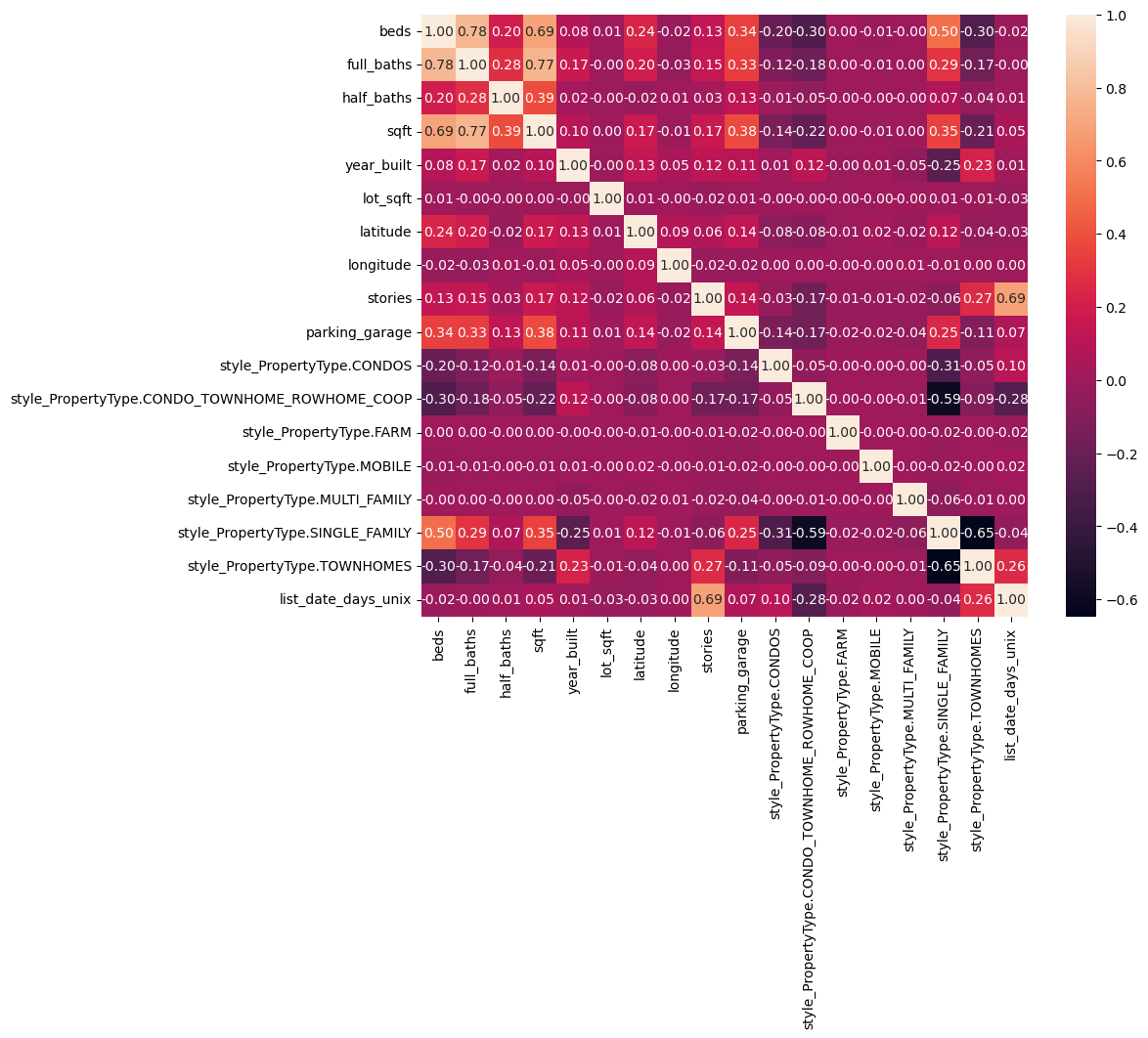
We one hot encoded the style feature because it is a categorical feature. Then, we converted list_date to the number of days since unix time so that we could treat it numerically. We looked at the correlation matrix for our features and saw that beds, full_baths, and other features were highly correlated, so we decided to test ridge regression along with linear regression. We then standardized the features and applied linear regression.
We chose linear regression as our ML algorithm to predict property prices. Since linear regression is a supervised learning method suitable for continuous data, it made sense to apply it to our target variable. We selected this model for its interpretability, as it easily allowed us to understand how different property attributes influence prices by looking at the weights of the model. Additionally, its computational efficiency and simplicity make it an excellent baseline model. We noticed that there were a couple of highly correlated features, so we decided to also test ridge regression.
Our RMSE for the two regressions was around 160,000, so we introduced polynomial features to better fit our data. Using polynomial features of degree 2, we were able to reduce RMSE to around 140,000. Higher degrees resulted in overfitting.
The following table displays results for polynomial degree 2:
| Best alpha | 6.7341506577508214 |
| Train RMSE | 149941.43291780588 |
| Test RMSE | 140464.64208894438 |
| Train RMSE Ridge | 152639.48486846185 |
| Test RMSE Ridge | 143193.17126680695 |
| Train R2 | 0.7871708164031062 |
| Test R2 | 0.8080459623798023 |
| Train R2 Ridge | 0.7794425922708255 |
| Test R2 Ridge | 0.8005161081147739 |
The following table displays results for polynomial degree 1:
| Best alpha | 351.11917342151276 |
| Train RMSE | 168714.003776309 |
| Test RMSE | 159313.80684948218 |
| Train RMSE Ridge | 168894.6141816911 |
| Test RMSE Ridge | 159715.8792556989 |
| Train R2 | 0.7305425912464059 |
| Test R2 | 0.7530721650984262 |
| Train R2 Ridge | 0.7299653675430132 |
| Test R2 Ridge | 0.7518242110813702xs |
Results and Discussion
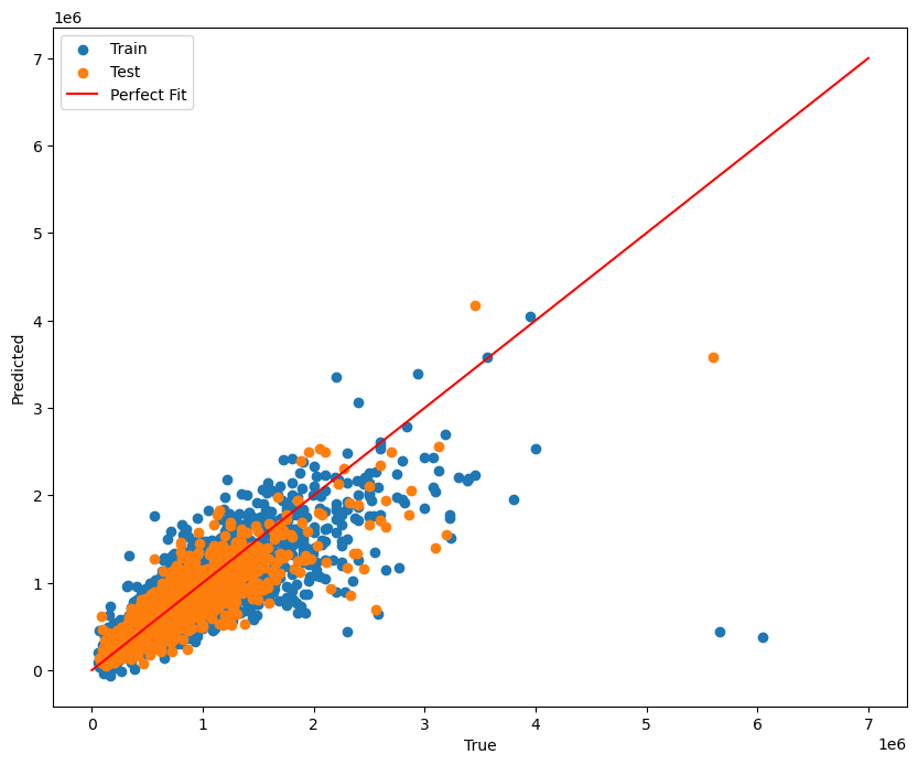
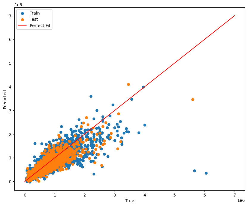
We had a high RMSE of around 140,000 for linear regression. Note that the mean house price is around 490,000. We suspect this is because the relationship between price and the features is nonlinear. We did try increasing the degrees of numerical features, but that helped only a little. However, our R^2 values for our models were around 0.8, which means the models have relatively good fit. Thus, the high RMSE value could be partially explained by some bad datapoint outliers that are disproportionately affecting RMSE (such as the points in the bottom right corner of the graph).
The following graphs show the results of linear and ridge regression, respectively.
 There are lots of points that are outliers from the linear regression line, which may explain the high RMSE.
 Similar to our linear regression model, there are lots of points that are outliers from the linear regression line, which may explain the high RMSE.
 This correlation heatmap shows the correlations between different features in the dataset, with lighter colors representing a strong correlation and vice versa.
One of our next steps includes using a different model like XGBoost to handle non-linear features. We could also first cluster the data using K-means and then apply a regression like Neural Networks or XGBoost to each individual cluster.
References
[1] F. Bergadano, R. Bertilone, D. Paolotti, and G. Ruffo, “Developing real estate automated valuation models by learning from heterogeneous data sources,” International Journal of Real Estate Studies, vol. 15, no. 1, pp. 72–85, Jun. 2021. doi:10.11113/intrest.v15n1.10
[2] G. Kamtziridis, D. Vrakas, and G. Tsoumakas, “Does noise affect housing prices? A case study in the urban area of Thessaloniki,” EPJ Data Science, vol. 12, no. 1, Oct. 2023. doi:10.1140/epjds/s13688-023-00424-3
[3] H. Sharma, H. Harsora, and B. Ogunleye, “An optimal house price prediction algorithm: Xgboost,” Journal of Analytics, vol. 3, no. 1, pp. 30–45, Jan. 2024. doi:10.3390/analytics3010003
GANTT Chart
Contribution Table
| Name | Contributions |
|---|---|
| Anh Dang | Data preprocessing, GitHub Pages |
| Arjun Brithi | Model Building |
| Ayush Gundawar | Model Building, Methods |
| Daniel Oh | Model Building |
| Jatong Su | Data preprocessing, Methods |