Final Report
Introduction
The accurate valuation of residential properties is a critical component in the real estate and mortgage lending industries, as it is influenced by both the physical attributes of the property and the characteristics of the surrounding neighborhood. Extensive research has been conducted to evaluate various machine learning techniques for predicting housing prices. A study titled “An Optimal House Price Prediction Algorithm: XGBoost” compared the performance of algorithms such as XGBoost, Support Vector Regressor, Random Forest Regressor, Multilayer Perceptron, and Multiple Linear Regression using the Ames City housing dataset.
The study identified XGBoost as the most effective model, offering interpretability, simplicity, and accuracy [3]. The dataset utilized in this analysis consists of property listings scraped from realtor.com, focusing on houses sold within the past decade in the area located around Duluth, Johns Creek, and Suwanee. The dataset includes features such as sale price, property location, year of construction, number of bedrooms, number of bathrooms, and other amenities that are crucial for determining property value. The inclusion of location details will facilitate future regional analysis [1].
Problem Definition
Accurate house pricing in Georgia’s dynamic real estate market poses a complex challenge. Traditional valuation methods, such as comparative market analysis, frequently overlook essential details and lack critical contextual information [2], resulting in frequent mispricing and discrepancies from true market value. Furthermore, obtaining more precise valuations can be time-consuming and costly. This project aims to address these limitations by leveraging machine learning models, which can analyze vast amounts of data to provide more precise and reliable property valuations.
Methods
Preprocessing
Initially, the data was cleansed by eliminating duplicate entries and imputing missing values. In the preprocessing phase, a selection was made to include only those features amenable to numerical representation for the training process. The original dataset comprised 29 columns, from which 12 pertinent features were retained after excluding irrelevant ones such as mls_id, property_url, and primary_photo.
The refined dataset comprised the following features: [status, style, street, city, zip_code, beds, full_baths, half_baths, sqft, year_built, days_on_mls, list_price, list_date, sold_price, last_sold_date, lot_sqft, price_per_sqft, latitude, longitude, stories, hoa_fee, parking_garage].
Categorical variables including status, style, street, city, and zip_code underwent one-hot encoding. Numerical features were cleansed of extreme outliers. The list_date was transformed into a numerical format representing the number of days since the Unix epoch, facilitating its use in quantitative analysis. Additionally, the age of the property was calculated by determining the interval between the current date and the year_built. Temporal attributes such as month, quarter, and year were derived from list_date to capture potential seasonal influences on the models. Subsequently, the features were standardized, and the dataset was divided into training and testing subsets.
Linear Regression
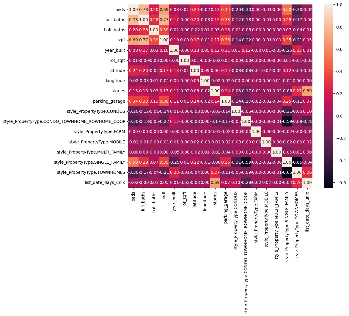
In our initial approach to predict property prices, we employed linear regression, a supervised learning algorithm suitable for continuous data such as housing prices. Upon examining the correlation matrix for our features, we observed that beds, full_baths, and other features exhibited high correlation. Consequently, we decided to test ridge regression alongside linear regression. The rationale behind selecting this model was its interpretability, as it facilitated an understanding of how different property attributes influence prices by examining the model’s weights. Additionally, its computational efficiency and simplicity made it an excellent baseline model.
To better fit our data and potentially achieve a lower root mean squared error (RMSE), we introduced polynomial features. By incorporating polynomial features of degree 2, we aimed to capture non-linear relationships present in the data. Through this approach, we were able to reduce the RMSE to approximately 140,000. However, higher degrees resulted in overfitting, prompting us to maintain the degree at 2 to strike a balance between model complexity and predictive performance.
Ridge Regression
In addition to linear regression, we explored ridge regression as an alternative model. This decision was prompted by the presence of highly correlated features, which can lead to instability in traditional linear regression models. Ridge regression, on the other hand, is adept at handling multicollinearity.
By employing regularization via ridge regression, we aimed to increase model stability and enhance its generalization ability. The regularization term aids in controlling the impact of highly correlated features on the prediction, a capability that linear regression lacks.
Random Forest
We also decided to employ Random Forest, a supervised machine learning algorithm, as it is capable of handling non-linear relationships and capturing more complex patterns in the data. Random Forest combines multiple decision trees during its training and averages their predictions, which typically leads to better accuracy and reduced overfitting compared to individual decision trees on their own. One of the main advantages of Random Forest is its suitability for real-world datasets that may have varying degrees of quality, as it is resistant to outliers, noisy data, and categorical features. Additionally, we can gain insights into which features are the most important when predicting house prices. By leveraging Random Forest, we aimed to utilize a model that can effectively handle non-linearities and interactions between features, potentially leading to better predictions than regression-based models.
XGBoost
The fourth machine learning algorithm employed to predict housing prices was XGBoost (Extreme Gradient Boosting), a supervised learning method that excels in regression tasks and is capable of handling complex datasets with high dimensionality. The rationale behind selecting XGBoost was its sequential training of weak decision trees to correct errors made by previous models. This iterative training process enables XGBoost to capture and learn more intricate patterns and interactions within the data, rendering it effective in modeling the relationships between house features and prices.
Additionally, XGBoost’s flexibility in handling missing values and categorical features further contributed to its appeal. Similar to Random Forest, XGBoost provides insights into the most important features, facilitating a comparative analysis between the models.
Results and Discussion
Linear Regression and Ridge Regression
The following table displays results for polynomial degree 2:
| Best alpha | 6.7341506577508214 |
| Train RMSE | 149941.43291780588 |
| Test RMSE | 140464.64208894438 |
| Train RMSE Ridge | 152639.48486846185 |
| Test RMSE Ridge | 143193.17126680695 |
| Train R2 | 0.7871708164031062 |
| Test R2 | 0.8080459623798023 |
| Train R2 Ridge | 0.7794425922708255 |
| Test R2 Ridge | 0.8005161081147739 |
The following table displays results for polynomial degree 1:
| Best alpha | 351.11917342151276 |
| Train RMSE | 168714.003776309 |
| Test RMSE | 159313.80684948218 |
| Train RMSE Ridge | 168894.6141816911 |
| Test RMSE Ridge | 159715.8792556989 |
| Train R2 | 0.7305425912464059 |
| Test R2 | 0.7530721650984262 |
| Train R2 Ridge | 0.7299653675430132 |
| Test R2 Ridge | 0.7518242110813702xs |
We had a high RMSE of around 140,000 for linear regression. Note that the mean house price is around 490,000. We suspect this is because the relationship between price and the features is nonlinear. We did try increasing the degrees of numerical features, but that helped only a little. However, our R^2 values for our models were around 0.8, which means the models have a relatively good fit. Thus, the high RMSE value could be partially explained by some bad datapoint outliers that are disproportionately affecting RMSE (such as the points in the bottom right corner of the graph).
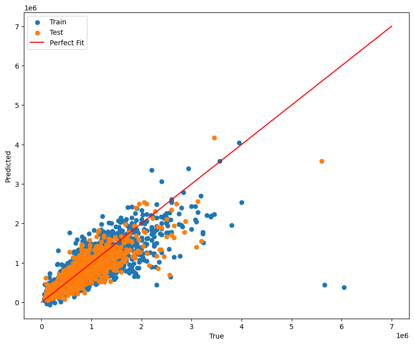
There are lots of points that are outliers from the linear regression line, which may explain the high RMSE.
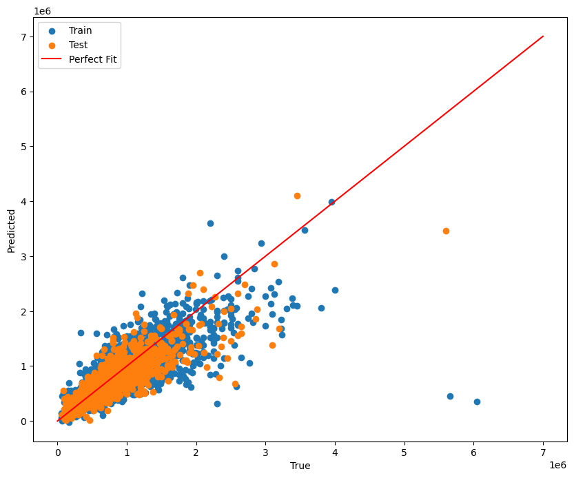
Similar to our linear regression model, there are lots of points that are outliers from the linear regression line, which may explain the high RMSE.
Random Forest
The following table displays the results for the random forest model:
| Training RMSE | 23723.302565932157 |
| Training R^2 | 0.9834086780073907 |
| Testing RMSE | 63990.71949090199 |
| Testing R^2 | 0.8802218333936377 |
Random Forest had a significantly lower RMSE on the training data than both the linear and ridge regression models, at around 24,000. However, there was a significant increase in the RMSE on the testing data, which strongly hints that there may be overfitting in this model. We can see that there was still a high R^2 of around 0.88, which suggests that despite struggling to generalize to some unseen data, the Random Forest model is generally able to capture variance in the dataset well.
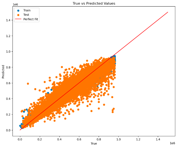
The perfect fit line is roughly along the middle, but there are still lots of data points in both sets that are far from it, showcasing why there may be a high RMSE.
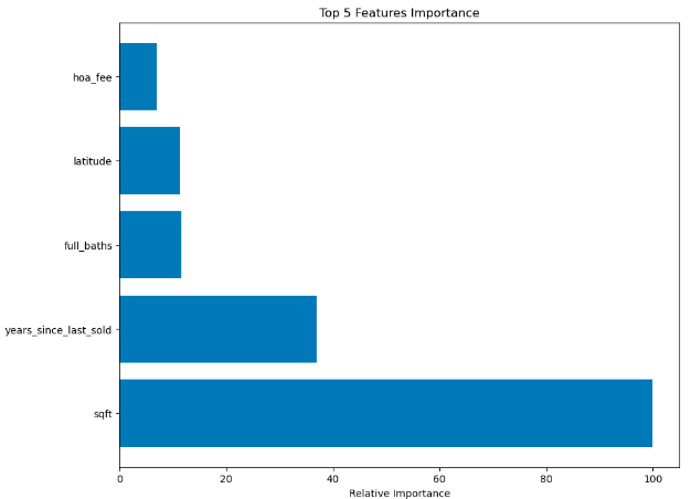
Relative Feature Importance - Random Forest provides insights into feature importance, allowing us to understand which features have the biggest impacts on housing price predictions. This information can be extremely valuable when weighing house purchasing decisions. Here, we see that square footage has, by far, the most relative importance out of all the features, with years since the last sale, full bathroom count, latitude (position), and HOA fees rounding out the top five.
XGBoost
The following table displays the results for the random forest model:
| Training RMSE | 50714.89595253979 |
| Training R^2 | 0.9241768585570102 |
| Testing RMSE | 61121.43043336859 |
| Testing R^2 | 0.8907225143598981 |
XGBoost had a relatively low RMSE on both the training and testing data, showing that it had a pretty strong performance overall. On the training data, the high R^2 of 0.92 and generally low RMSE of around 51,000 suggests that the XGBoost model was a good fit for the training data. On the testing data, the R^2 slightly decreased to around 0.89, and the RMSE slightly increased to around 61,000, implying a somewhat worse fit, but the numbers are quite similar overall. Compared to previous models, XGBoost does not seem to struggle with generalizing as much, although there is still a slight discrepancy between the two results. Nonetheless, its low RMSE and high R^2 indicate XGBoost’s ability to effectively learn patterns and relationships within the data.
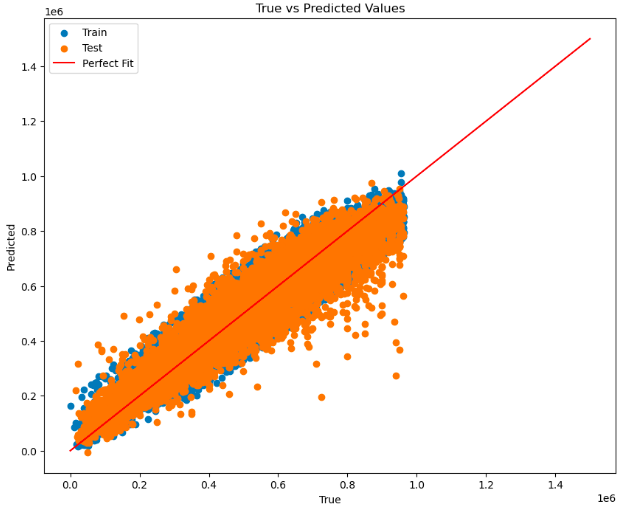
The perfect fit line aligns approximately with the middle of the data distribution, yet the numerous data points that significantly deviate from it contribute to the high RMSE, especially in the (relatively higher RMSE) testing data.
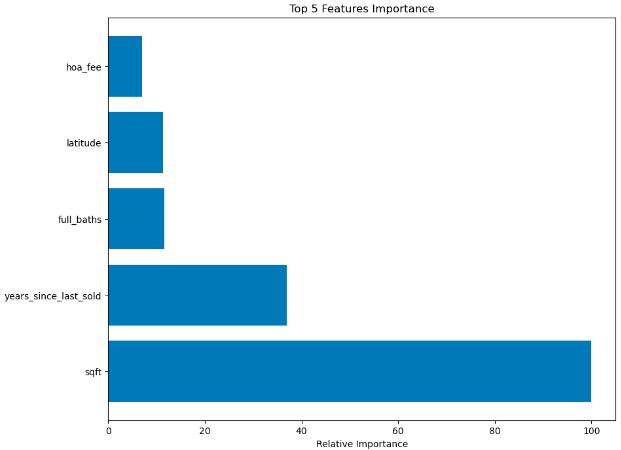
Similarly to Random Forest, XGBoost provides us with a relative feature importance table. Again, the most important feature is square footage, and the rest of the top five is the same.
Feature Correlation
This correlation heatmap shows the correlations between different features in the dataset, with lighter colors representing a strong correlation and vice versa.
Comparison and Next Steps
Among the four models analyzed, XGBoost distinguished itself with its balanced performance across both training and testing datasets. The comparative analysis of the models highlights specific trade-offs and strengths. Linear Regression and Ridge Regression, while providing interpretability and resistance to multicollinearity, respectively, were less effective in capturing non-linear relationships, resulting in higher RMSE values. Conversely, Random Forest achieved a lower RMSE during training but exhibited signs of overfitting as evidenced by the disparity between its training and testing outcomes, underscoring the necessity of meticulous hyperparameter tuning. Nevertheless, its ability to address non-linear relationships and offer insights into feature importance remains valuable.
XGBoost, however, demonstrated superior overall performance with low RMSE and high R-squared values across both datasets, indicating better generalization capabilities compared to Random Forest. Its proficiency in managing complex data, missing values, and categorical features further enhanced its utility.
Despite their respective strengths, each model encountered challenges in accurately predicting housing prices within the complexities of the real estate market.
Future initiatives will focus on refining hyperparameters for the Random Forest and XGBoost models, advancing feature engineering techniques to derive more significant data insights, exploring ensemble methods such as stacking and blending to augment accuracy and incorporating external factors like market trends and economic indicators into our analysis.
References
[1] F. Bergadano, R. Bertilone, D. Paolotti, and G. Ruffo, “Developing real estate automated valuation models by learning from heterogeneous data sources,” International Journal of Real Estate Studies, vol. 15, no. 1, pp. 72–85, Jun. 2021. doi:10.11113/intrest.v15n1.10
[2] G. Kamtziridis, D. Vrakas, and G. Tsoumakas, “Does noise affect housing prices? A case study in the urban area of Thessaloniki,” EPJ Data Science, vol. 12, no. 1, Oct. 2023. doi:10.1140/epjds/s13688-023-00424-3
[3] H. Sharma, H. Harsora, and B. Ogunleye, “An optimal house price prediction algorithm: Xgboost,” Journal of Analytics, vol. 3, no. 1, pp. 30–45, Jan. 2024. doi:10.3390/analytics3010003
Presentation Video
GANTT Chart
Contribution Table
| Name | Contributions |
|---|---|
| Anh Dang | Video (editing, narration), GitHub Pages |
| Arjun Brithi | Video (slides, script), models |
| Ayush Gundawar | Models (Random Forest) |
| Daniel Oh | Video (editing, narration) |
| Jatong Su | Models (XGBoost) |